First overview of a measurement
Measuring NMR spectra of samples often results in a series of measurements, and one of the first tasks is to get an overview what has been measured and how the results look like.
Classes used:
Processing
Plotting
Recipe
Complete recipe for getting an overview and compare two spectra.
 1format:
 2  type: ASpecD recipe
 3  version: '0.2'
 4settings:
 5  default_package: nmraspecds
 6directories:
 7  datasets_source: ../../tests/testdata/
 8datasets:
 9- source: Adamantane/1
10  id: 1H
11  importer_parameter:
12    processing_number: 2
13- source: Adamantane/2
14  id: 13C
15tasks:
16  - kind: singleplot
17    type: SinglePlotter1D
18    properties:
19      properties:
20        figure:
21          dpi: 600
22      filename:
23        - ProtonSpectrum.png
24        - CarbonSpectrum.png
25  - kind: processing
26    type: Normalisation
27  - kind: multiplot
28    type: MultiPlotter1D
29    properties:
30      properties:
31        figure:
32          dpi: 600
33        axes:
34          xlim: [100, -100]
35      parameters:
36        offset: 1
37      filename: BothSpectra.png
38    apply_to:
39      - 13C
40      - 1H
Result

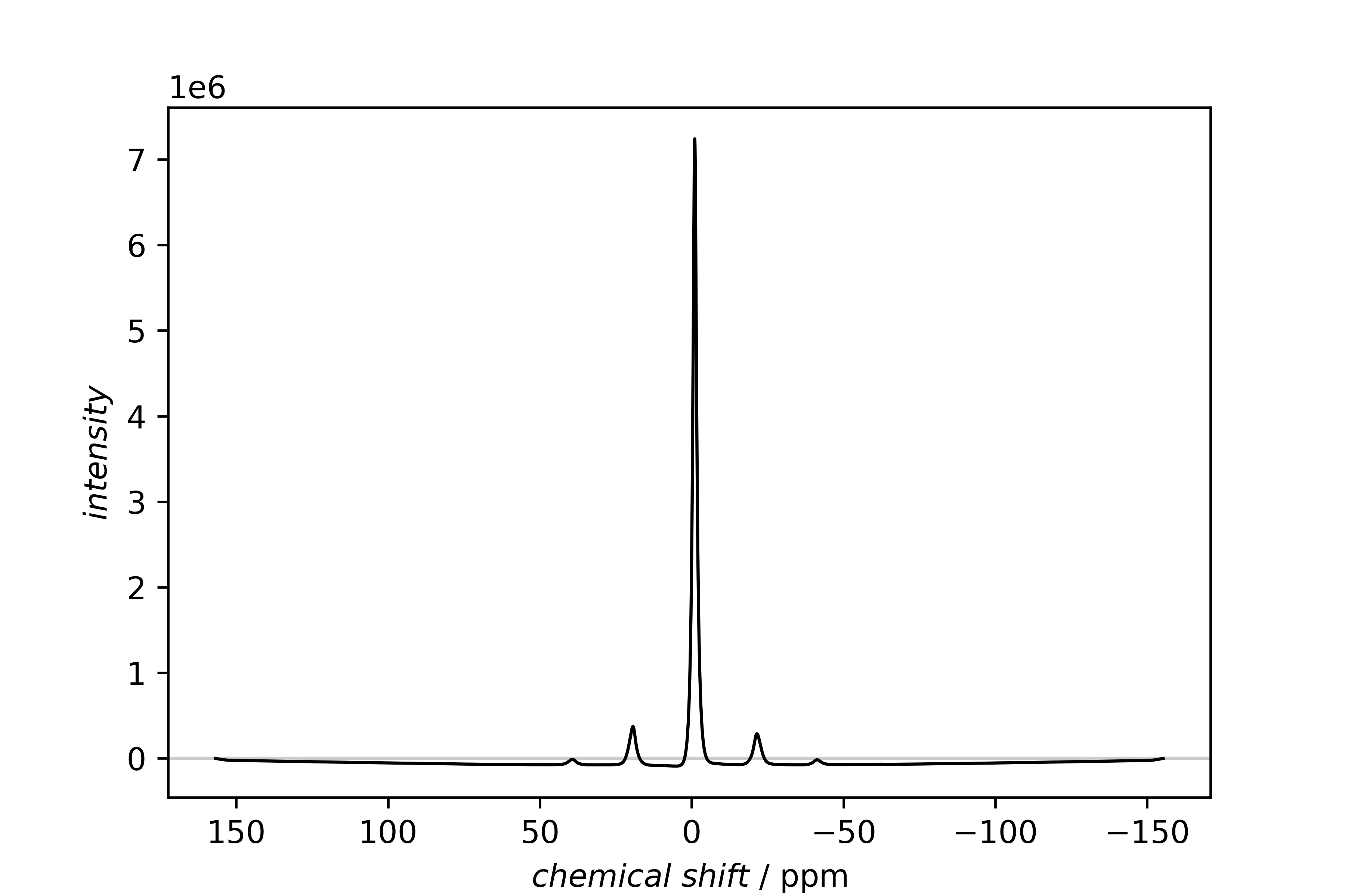
1H spectrum

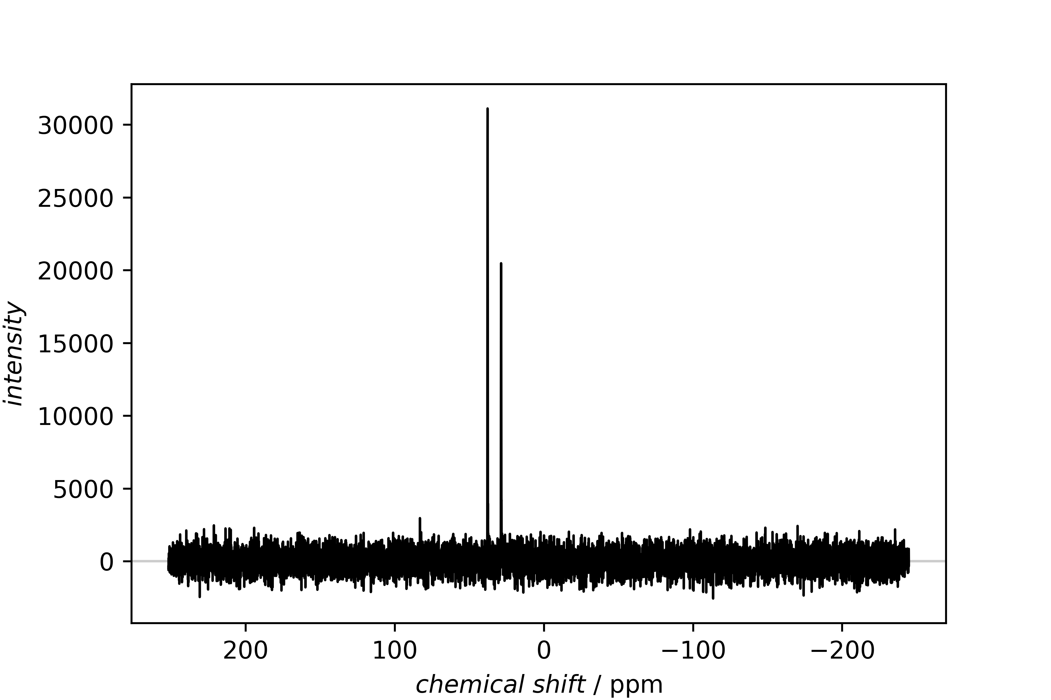
13C spectrum

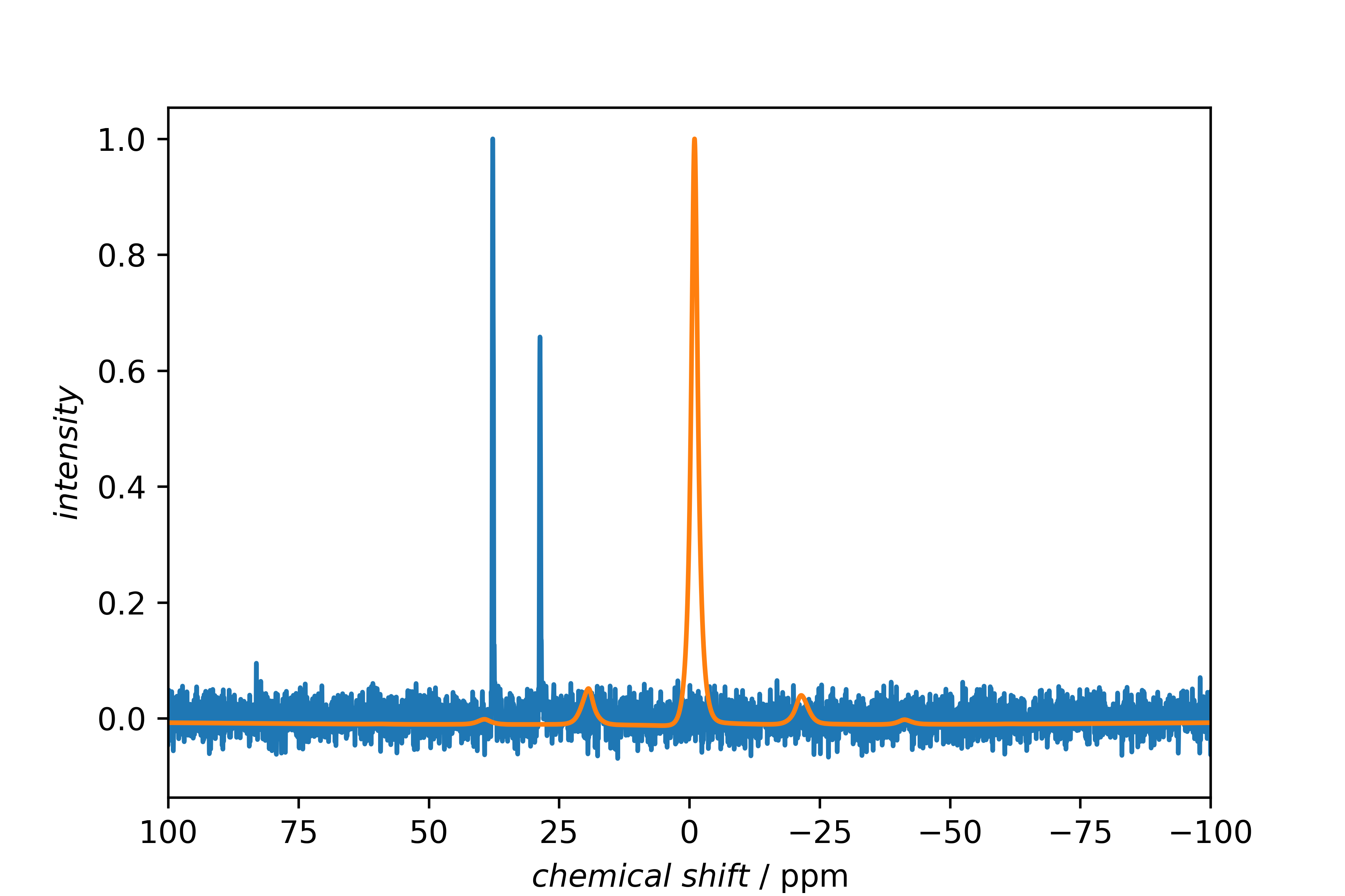
Both spectra in one figure.
Comments
The recipe starts with information about its version, the default package and the source path of the datasets.
At the import, the second processing number is called for the 1H dataset, indicated by the importer_parameter keyword.
The 13C data is imported without any further parameters, meaning, that the first processing number is imported
Both datasets get an ID with which they are called later.
Directly after the import, both spectra are plotted separately with the SinglePlotter1D.
Then, they are normalized, without further parameters, this is done using the maximum.
Both spectra are plotted into one figure (ignoring that plotting a 1H spectrum over a 13C spectrum physically makes nearly no sense).